temp <- tempfile()
download_url <- "https://userpage.fu-berlin.de/soga/data/raw-data/spatial/"
zipfile <- "berlin-latest-free.shp.zip"

## download the file
download.file(paste0(download_url, zipfile), temp, mode = "wb")
## unzip the file(s)
unzip(temp, exdir = "data")

## close file connection
unlink(temp)1 Introduction
The map on the cover of this article shows transit travel times from 189 hotel clusters to 50 cultural and nightlife destinations across Berlin. Each hexagon is shaded by average travel time; the isolines mark 5-minute intervals; the red circles are 1, 3, and 5 km from the geographic centre. The point it makes is geographic: transit accessibility and physical proximity are different things.
This article is about how that map was built. The motivating problem was a hotel search analysis — ranking hotels by transit time to a traveller’s specific points of interest rather than by distance from the city centre. But the pipeline generalises to any problem where you need to measure accessibility between a set of origins and destinations at city scale: venue analysis, urban planning, catchment area modelling.
Three engineering decisions shape the structure. First, how to reduce 22,750 potential routing requests to something tractable without losing spatial resolution — that’s the H3 clustering section. Second, how to run thousands of API calls in a loop that doesn’t die on the network error and doesn’t create a memory bottleneck as results accumulate — that’s the routing loop section. Third, how to turn a sparse set of point measurements into a readable continuous surface with labelled isolines over a basemap — that’s the visualisation section.
The code is in R. The libraries doing the work are h3jsr for hexagonal indexing, gmapsdistance for routing, gstat and stars for IDW interpolation, and metR and ggspatial for the final map composition.
2 Load Data
The source data comes from the OpenStreetMap extract for Berlin via Freie Universität Berlin, containing features such as museums, theaters, parks, and other attractions.
library(sf)

berlin_features <- st_read("data/gis_osm_pois_free_1.shp", quiet = TRUE)
berlin_features |> glimpse()
Rows: 83,123
Columns: 5
$ osm_id <chr> "16541597", "26735749", "26735753", "26735759", "26735763", "…
$ code <int> 2907, 2301, 2006, 2301, 2301, 2701, 2307, 2031, 2724, 2907, 2…
$ fclass <chr> "camera_surveillance", "restaurant", "telephone", "restaurant…
$ name <chr> "Aral", "Aida", NA, "Madame Ngo", "Thanh Long", NA, "Spinnerb…
$ geometry <POINT [°]> POINT (13.34544 52.54644), POINT (13.32282 52.50691), P…3 Explore POI Data
The OSM extract contains dozens of feature classes. We need to narrow to the ones that represent meaningful destinations for a visitor: cultural venues, nightlife, landmarks, and exclude noise like parking lots and post boxes.
berlin_features$fclass |> unique() |> sort() [1] "archaeological" "arts_centre" "artwork"
[4] "atm" "attraction" "bakery"
[7] "bank" "bar" "battlefield"
[10] "beauty_shop" "bench" "beverages"
[13] "bicycle_rental" "bicycle_shop" "biergarten"
[16] "bookshop" "butcher" "cafe"
[19] "camera_surveillance" "camp_site" "car_dealership"
[22] "car_rental" "car_sharing" "car_wash"
[25] "caravan_site" "chalet" "chemist"
[28] "cinema" "clinic" "clothes"
[31] "college" "comms_tower" "community_centre"
[34] "computer_shop" "convenience" "courthouse"
[37] "dentist" "department_store" "doctors"
[40] "dog_park" "doityourself" "drinking_water"
[43] "embassy" "fast_food" "fire_station"
[46] "florist" "food_court" "fountain"
[49] "furniture_shop" "garden_centre" "general"
[52] "gift_shop" "golf_course" "graveyard"
[55] "greengrocer" "guesthouse" "hairdresser"
[58] "hospital" "hostel" "hotel"
[61] "hunting_stand" "jeweller" "kindergarten"
[64] "kiosk" "laundry" "library"
[67] "mall" "market_place" "memorial"
[70] "mobile_phone_shop" "monument" "motel"
[73] "museum" "newsagent" "nightclub"
[76] "nursing_home" "observation_tower" "optician"
[79] "outdoor_shop" "park" "pharmacy"
[82] "picnic_site" "pitch" "playground"
[85] "police" "post_box" "post_office"
[88] "prison" "pub" "recycling"
[91] "recycling_clothes" "recycling_glass" "recycling_paper"
[94] "restaurant" "ruins" "school"
[97] "shelter" "shoe_shop" "sports_centre"
[100] "sports_shop" "stadium" "stationery"
[103] "supermarket" "swimming_pool" "telephone"
[106] "theatre" "theme_park" "toilet"
[109] "tourist_info" "tower" "town_hall"
[112] "toy_shop" "track" "travel_agent"
[115] "university" "vending_any" "vending_cigarette"
[118] "vending_machine" "vending_parking" "veterinary"
[121] "video_shop" "viewpoint" "waste_basket"
[124] "water_mill" "water_tower" "water_well"
[127] "water_works" "wayside_cross" "wayside_shrine"
[130] "zoo" poi_classes <- c("archaeological", "attraction", "monument",
"museum", "nightclub", "observation_tower", "ruins",
"graveyard", "stadium", "theatre", "zoo"
)
berlin_pois <- berlin_features |> filter(fclass %in% poi_classes)
berlin_pois |> glimpse()Rows: 495
Columns: 5
$ osm_id <chr> "66917094", "66917098", "66917115", "66917188", "73696610", "…
$ code <int> 2201, 2201, 2201, 2201, 2722, 2201, 2722, 2201, 2721, 2201, 2…
$ fclass <chr> "theatre", "theatre", "theatre", "theatre", "museum", "theatr…
$ name <chr> "Friedrichstadt-Palast", "Quatsch Comedy Club", "Kabarett-The…
$ geometry <POINT [°]> POINT (13.38888 52.52392), POINT (13.38862 52.52362), P…library(ggplot2)
library(sf)
library(ggspatial)
berlin_pois <- berlin_pois |> mutate(
loc = st_coordinates(geometry),
coord = map2(loc[,2], loc[,1], ~c(.x, .y))
) |> select(-loc) |> as.data.frame()
berlin_pois$lng <- berlin_pois$coord |> map_dbl(2)
berlin_pois$lat <- berlin_pois$coord |> map_dbl(1)
berlin_pois_sf <- berlin_pois |>
sample_n(100) |>
st_as_sf(coords = c("lng", "lat"), crs = 4326)
ggplot() +
annotation_map_tile(type = "osm", zoom = 12) +
geom_sf(data = st_transform(berlin_pois_sf, 3857),
color = "purple",
size = 2) +
theme_minimal() +
theme(
axis.text = element_blank(),
axis.title = element_blank()
) +
labs(
title = "Berlin POIs by Category",
subtitle = "Cultural and nightlife locations"
)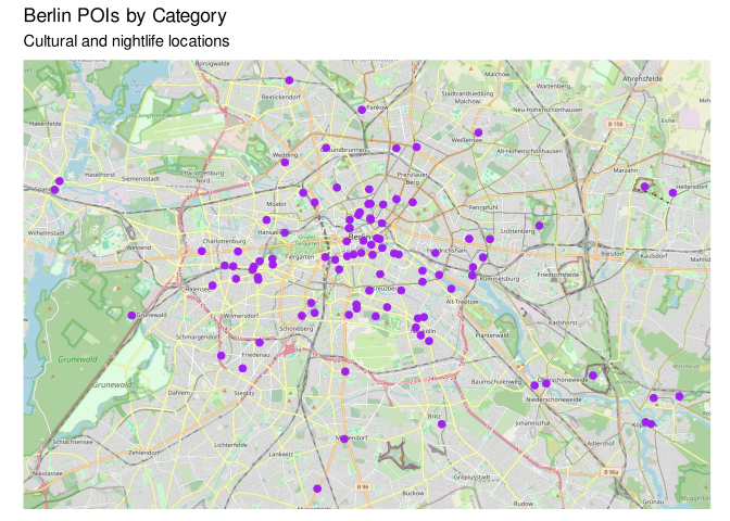
With all 11 POI classes included, the points are scattered across the map forming no visible clusters. The next step is to rank by engagement and trim to the destinations that are popular among travellers.
4 Add Reviews Data to POIs
Google Places ratings serve as a proxy for a POI’s relevance: places with more reviews have been visited by more people. It worth noting that ratings follow a heavily right-skewed distribution. The Berlin Zoo has hundreds of thousands of reviews; a small neighbourhood museum might have 800. Filtering naively by the top 50 on raw count produces a list dominated by mass-market tourist attractions, which are already well-served by central hotels. For the scenario-based analysis here this is manageable, but a general-purpose accessibility ranking would need a more careful POI selection methodology.
berlin_pois <- berlin_pois |> mutate(
  loc = st_coordinates(geometry),
  coord = map2(loc[,2], loc[,1], ~c(.x, .y))
) |> select(-loc) |> as.data.frame()

berlin_pois |> glimpse()
Rows: 495
Columns: 8
$ osm_id <chr> "66917094", "66917098", "66917115", "66917188", "73696610", "…
$ code <int> 2201, 2201, 2201, 2201, 2722, 2201, 2722, 2201, 2721, 2201, 2…
$ fclass <chr> "theatre", "theatre", "theatre", "theatre", "museum", "theatr…
$ name <chr> "Friedrichstadt-Palast", "Quatsch Comedy Club", "Kabarett-The…
$ coord <list> <52.52392, 13.38888>, <52.52362, 13.38862>, <52.52067, 13.38…
$ geometry <POINT [°]> POINT (13.38888 52.52392), POINT (13.38862 52.52362), P…
$ lng <dbl> 13.38888, 13.38862, 13.38851, 13.38890, 13.36299, 13.27075, 1…
$ lat <dbl> 52.52392, 52.52362, 52.52067, 52.52077, 52.50761, 52.50887, 5…Here we set up the function to get the total number of user ratings for a given POI using the Google Places API. The function first performs a text search to find the place ID based on the name.
dotenv::load_dot_env()
api_key = Sys.getenv("GOOGLE_API_KEY")

library(googleway)

get_ratings_total <- function(place_name, coord, api_key) {
  res <- google_places(
    search_string = place_name,
    location = coord,
    key = api_key
  )

  res <- google_place_details(
    place_id = res$results$place_id[1],
    key = api_key
  )
  if( "user_ratings_total" %in% names(res$result) ) {
    res$result$user_ratings_total
  } else {
    0
  }
}
Let’s test the function on a few known POIs to confirm it’s working correctly before applying it to the entire dataset. We can compare the results to the Google Maps app for validation.
berlin_pois |>
  filter(name %in%
    c(
      "Friedrichstadt-Palast",
      "Quatsch Comedy Club",
      "Nordamerikanischer Baumstachler"
    )) |>
  rowwise() |>
  mutate(
    user_ratings_total =
      tryCatch(
        get_ratings_total(name, coord, api_key),
        error = function(e) {
          NA
        }
      )
  ) |>
ungroup() |> kable()| osm_id | code | fclass | name | coord | geometry | lng | lat | user_ratings_total |
|---|---|---|---|---|---|---|---|---|
| 66917094 | 2201 | theatre | Friedrichstadt-Palast | 52.52392, 13.38888 | POINT (13.38888 52.52392) | 13.38888 | 52.52392 | 24143 |
| 66917098 | 2201 | theatre | Quatsch Comedy Club | 52.52362, 13.38862 | POINT (13.38862 52.52362) | 13.38862 | 52.52362 | 2780 |
| 5637127166 | 2721 | attraction | Nordamerikanischer Baumstachler | 52.49811, 13.52441 | POINT (13.52441 52.49811) | 13.52441 | 52.49811 | 30664 |
The result matches the Google Maps app, confirming that the geocoding and place.id resolution are working correctly.
Warning
Executing the next chunk of code may take a few minutes due to the number of API calls and the 100ms sleep between them to respect rate limits. It will fall under the free tier of 10,000 calls of Google Maps API, but if you re-run it multiple times or scale up the number of POIs or hotels, you may incur costs. Consider caching results or using a smaller sample for testing. Google Maps pricing details can be found here.
The tryCatch ensures that if any individual POI lookup fails (due to rate limits, geocoding issues, or network errors), the loop continues and the failed POI gets an NA for its user_ratings_total, which can be filtered out later.
The resulting berlin_pois dataframe will have a new column user_ratings_total with the total number of user ratings for each POI, which can be used for filtering and weighting in the subsequent analysis.
berlin_pois <- berlin_pois |>
  rowwise() |>
  mutate(
    user_ratings_total =
      tryCatch(
        get_ratings_total(name, coord, api_key),
        error = function(e) { NA }
      )
  ) |>
  ungroup() |> kable()
Once we have the ratings data, we save the enriched POI dataset to disk. This allows us to avoid re-running the API calls in future sessions, which is useful given the time and cost associated with those calls.
berlin_pois |> saveRDS("data/berlin_pois_with_ratings.rds")The log scale on the histogram below is diagnostic; it shows the shape of the distribution without compressing the long tail into invisibility. The filtering itself still operates on the raw count.
berlin_pois <- readRDS("data/berlin_pois_with_ratings.rds")

ggplot(berlin_pois, aes(x = log1p(user_ratings_total))) +
  geom_histogram(fill = "lightblue", color = "black") +
  labs(
    title = "Distribution of User Ratings Total for POIs",
    x = "User Ratings Total",
    y = "Count"
  ) +
  scale_x_continuous(
    breaks = scales::pretty_breaks(n = 10),
    labels = function(x) round(expm1(x))
  ) +
  theme_minimal()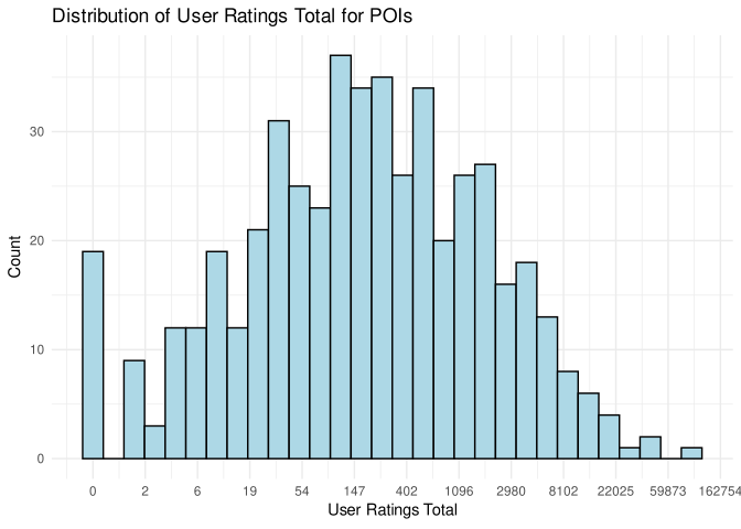
5 Select Popular POIs
berlin_pois <- berlin_pois |>
  sort_by(desc(berlin_pois$user_ratings_total))

berlin_pois |>
  head(10) |>
select(name, fclass, user_ratings_total) |> kable() | name | fclass | user_ratings_total |
|---|---|---|
| Checkpoint Charlie | attraction | 93856 |
| Tresorfabrik Arnheim | attraction | 40160 |
| Topographie des Terrors | attraction | 39712 |
| Schloss Charlottenburg | museum | 30564 |
| Friedrichstadt-Palast | theatre | 23359 |
| Madame Tussauds | museum | 21861 |
| Puro Sky Lounge Berlin | nightclub | 20583 |
| Deutsches Spionagemuseum | museum | 18614 |
| Freies Museum Berlin e.V. | museum | 12430 |
| Berliner Unterwelten-Museum | museum | 12403 |
Note
What is “Tresorfabrik Arnheim” by the way? A quick Google search suggests the Tresorfabrik S. J. Arnheim (founded in 1833) was the first and largest manufacturer of safes and vaults in Germany, located in the Berlin district of Wedding. Either most of those 40,160 Google reviews are from the 19th century, or the ratings belong to a different attraction. Let’s exclude it from the results. We probably should have started the search with the Google Maps API to avoid this kind of error.
Let’s see how the top 50 POIs are distributed across classes.
# Exclude Tresorfabrik Arnheim
berlin_pois <- berlin_pois |>
  filter(name != "Tresorfabrik Arnheim")
# Check class distribution of top 50 POIs
berlin_pois |>
  head(50) |>
group_by(fclass) |> count() |> kable()| fclass | n |
|---|---|
| attraction | 5 |
| museum | 23 |
| nightclub | 13 |
| ruins | 1 |
| theatre | 8 |
library(ggplot2)
library(sf)
library(ggspatial)

berlin_pois$lng <- berlin_pois$coord |> map_dbl(2)
berlin_pois$lat <- berlin_pois$coord |> map_dbl(1)

berlin_pois_sf <- berlin_pois |>
  head(50) |>
  st_as_sf(coords = c("lng", "lat"), crs = 4326)

poi_shapes <- c(
  "attraction" = 17,
  "museum"     = 15,
  "theatre"    = 18,
  "nightclub"  = 19,
  "ruins"      = 8
)

poi_colors <- c(
  "attraction" = "#E41A1C",
  "museum"     = "#377EB8",
  "theatre"    = "#4DAF4A",
  "nightclub"  = "#984EA3",
  "ruins"      = "#FF7F00"
)

ggplot() +
  annotation_map_tile(type = "osm", zoom = 12) +
  geom_sf(data = st_transform(berlin_pois_sf, 3857),
          aes(shape = fclass, color = fclass),
          size = 3) +
  scale_shape_manual(values = poi_shapes, name = "Category") +
  scale_color_manual(values = poi_colors, name = "Category") +
  theme_minimal() +
  theme(
    axis.text = element_blank(),
    axis.title = element_blank(),
  ) +
  labs(
    title = "Berlin POIs by Category",
    subtitle = "Custom markers for cultural and nightlife locations"
  ) +
  theme(legend.position = "right")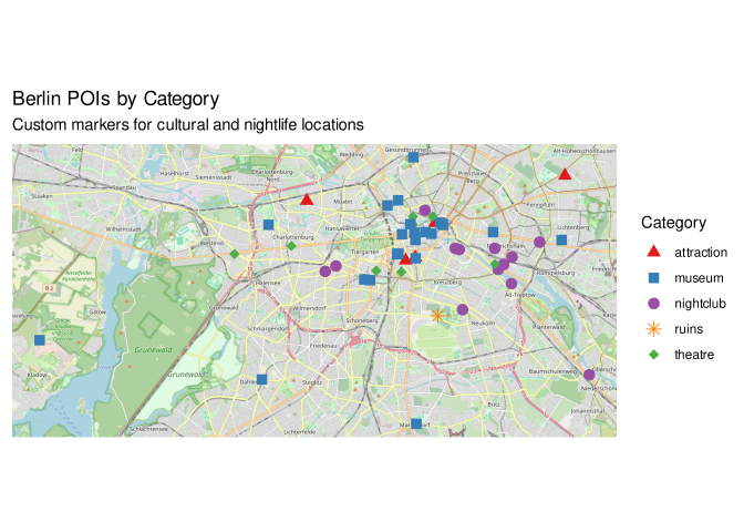
The spatial distribution is well-suited for the analysis — POIs are not concentrated purely at the centre, so the transit time signal will vary meaningfully across the hotel map.
berlin_pois <- berlin_pois |> head(50)6 Collect Hotel Locations
hotels <- berlin_features |>
  filter(fclass == "hotel") |>
  select(osm_id, name, geometry)

hotels |> glimpse()
Rows: 455
Columns: 3
$ osm_id <chr> "58467591", "60105926", "60105927", "60105928", "60237649", "…
$ name <chr> "Park Plaza Wallstreet", "Living Hotel Großer Kurfürst", "art…
$ geometry <POINT [°]> POINT (13.4078 52.51146), POINT (13.40879 52.51225), PO…What about the spatial distribution of hotels? Are they clustered in a few neighbourhoods, or spread evenly across the city? This will inform the clustering strategy for routing.
library(ggplot2)
library(sf)
library(ggspatial)

hotels <- hotels |> mutate(
  loc = st_coordinates(geometry),
  coord = map2(loc[,2], loc[,1], ~c(.x, .y))
) |> select(-loc) |> as.data.frame()

hotels$lng <- hotels$coord |> map_dbl(2)
hotels$lat <- hotels$coord |> map_dbl(1)

hotels_sf <- hotels |>
  st_as_sf(coords = c("lng", "lat"), crs = 4326)

ggplot() +
  annotation_map_tile(type = "osm", zoom = 12) +
  geom_sf(
    data = st_transform(hotels_sf, 3857), color = "red", size = 2
  ) +
  theme_minimal() +
  theme(
    axis.text = element_blank(),
    axis.title = element_blank(),
  ) +
  labs(
    title = "Berlin Hotels"
  )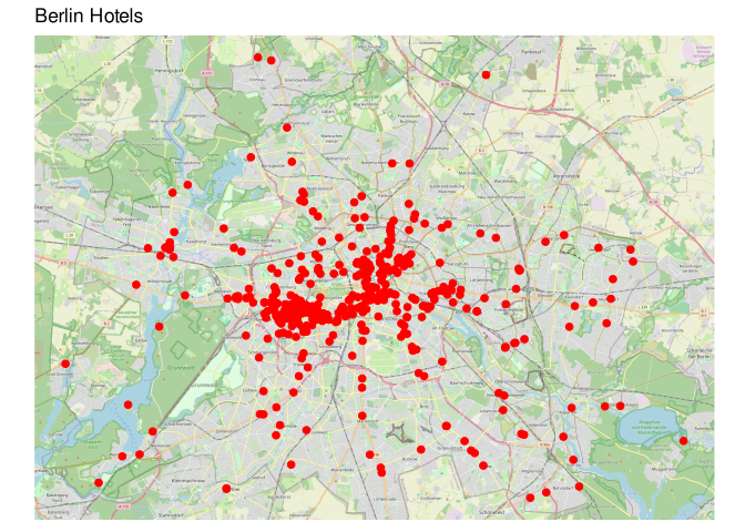
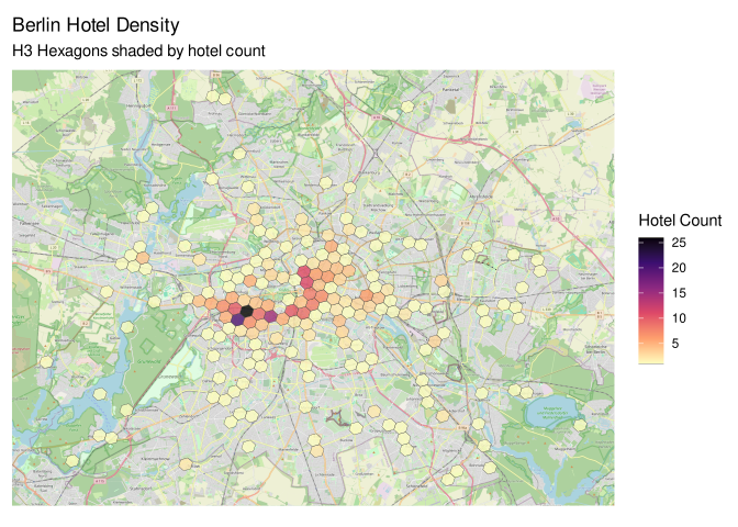
455 hotels × 50 POIs = 22,750 routing requests. At Google Maps Distance Matrix API pricing that’s non-trivial, and the time cost of 100ms sleep between calls makes it impractical to run in full. Clustering reduces both cost and runtime. Failure handling is a separate concern — that’s what the tryCatch in the loop is for.
6.1 Cluster Hotels with H3
We cluster hotels using H3 — Uber’s hexagonal hierarchical geospatial indexing system. Each hotel is assigned to its hexagonal cell at a given resolution; hotels sharing a cell are represented by the cell centroid for routing. The choice of hexagons over a regular square grid is geometric: in a square cell, the distance from the centre to a corner is \(\sqrt{2}\) times the distance from the centre to an edge midpoint. In a regular hexagon, the centre-to-edge distance is constant on all six sides. For a routing approximation where the centroid stands in for every point in the cell, that uniformity matters — the maximum positional error is bounded and consistent, regardless of where within the cell a hotel actually sits.
library(h3jsr)

hotels <- hotels |>
  mutate(
    h3_index = point_to_cell(geometry, res = 8)
  )

hotels_h3 <- hotels |>
  select(h3_index, geometry) |>
  group_by(h3_index) |>
  summarise(
    hotel_count = n(),
    geometry = cell_to_polygon(h3_index)
  ) |> distinct()

hotels_h3 |> glimpse()
Rows: 189
Columns: 3
Groups: h3_index [189]
$ h3_index <chr> "881f188443fffff", "881f188455fffff", "881f188461fffff", "…
$ hotel_count <int> 1, 1, 1, 2, 1, 1, 1, 1, 1, 1, 2, 1, 1, 1, 1, 1, 1, 1, 2, 1…
$ geometry <POLYGON [°]> POLYGON ((13.1582 52.42471,..., POLYGON ((13.171 5…At resolution 8, cells have a mean area of approximately 0.74 km², reducing 455 hotels to 189 unique cells and cutting API calls by more than half.
library(ggplot2)
library(sf)
library(ggspatial)

hotels_h3_sf <- st_as_sf(hotels_h3) |>
  st_transform(3857)

ggplot() +
  annotation_map_tile(type = "osm", zoom = 12) +
  geom_sf(
    data = hotels_h3_sf,
    aes(fill = hotel_count),
    color = "#333333",
    linewidth = 0.1,
    alpha = 0.8
  ) +
  scale_fill_viridis_c(
    option = "magma",
    name = "Hotel Count", direction = -1
  ) +
  theme_minimal() +
  theme(
    axis.title = element_blank(),
    axis.text = element_blank(),
    axis.ticks = element_blank()
  ) +
  labs(
    title = "Berlin Hotel Density",
    subtitle = "H3 Hexagons shaded by hotel count"
  )
189 origins × 50 destinations = 9,450 routing requests. Manageable.
hotels_h3 <- hotels_h3 |>
  mutate(
    center = h3jsr::cell_to_point(h3_index)
  )

hotels_h3 <- hotels_h3 |>
  rowwise() |>
  mutate(
    center = st_coordinates(center),
    lat = center[,2],
    lng = center[,1]
  ) |>
  select(-center) |>
  distinct()

hotels_h3 |> glimpse()
Rows: 189
Columns: 5
Rowwise: h3_index
$ h3_index <chr> "881f188443fffff", "881f188455fffff", "881f188461fffff", "…
$ hotel_count <int> 1, 1, 1, 2, 1, 1, 1, 1, 1, 1, 2, 1, 1, 1, 1, 1, 1, 1, 2, 1…
$ geometry <POLYGON [°]> POLYGON ((13.1582 52.42471,..., POLYGON ((13.171 5…
$ lat <dbl> 52.42175, 52.42009, 52.40511, 52.40287, 52.44892, 52.44666…
$ lng <dbl> 13.16350, 13.17630, 13.13443, 13.25621, 13.16387, 13.28574…7 Calculate Travel Times
hotels_h3 <- hotels_h3 |>
  mutate(
    origin = paste0(lat, ", ", lng)
  )

origins <- hotels_h3 |>
  pull(origin) |>
  unique()

berlin_pois <- berlin_pois |>
  mutate(
    dest = paste0(
      st_coordinates(geometry)[, 2],
      ", ",
      st_coordinates(geometry)[, 1]
    )
  )

destinations <- berlin_pois |>
  head(50) |>
  pull(dest) |>
  unique()

paste("Number of origins:", length(origins))
[1] "Number of origins: 189"paste("Number of destinations:", length(destinations))[1] "Number of destinations: 50"The loop wraps each request in tryCatch as the Google Maps API occasionally returns errors on rate limit spikes, ambiguous geocoding, or network timeouts, and a bare for loop dies on the first one. The results are collected into a pre-allocated list rather than grown with rbind: rbind inside a loop copies the entire growing dataframe on every iteration, an \(O(n^2)\) memory pattern that is tolerable at 9,450 pairs but becomes the bottleneck if you scale to a larger city or expand the POI set. idx is incremented outside the tryCatch so failed pairs leave a NULL in the list; bind_rows drops NULLs silently.
Warning
The next code chunk makes 9,450 API calls to Google Maps. This may take several minutes to run and could incur costs if you exceed the free tier limits (see pricing info here). Consider caching results or using a smaller sample for testing.
library(ggmap)
library(gmapsdistance)

set.api.key(api_key)

# Pre-allocate a list to avoid rbind() inside the loop.
# rbind() copies the growing dataframe on every iteration — O(n²) memory
# behaviour that becomes noticeable above ~5k rows.
n_pairs <- length(origins) * length(destinations)
results_list <- vector("list", n_pairs)
idx <- 1

for (origin in origins) {
  for (destination in destinations) {
    tryCatch(
      {
        Sys.sleep(0.1)
        result <- gmapsdistance(
          origin      = origin,
          destination = destination,
          mode        = "transit"
        )
        results_list[[idx]] <- data.frame(
          origin      = origin,
          destination = destination,
          distance    = result$Distance,
          time        = result$Time
        )
      },
      error = function(e) {
        message(paste(
          "Error calculating travel time from", origin,
          "to", destination, ":", e$message
        ))
      }
    )
    idx <- idx + 1  # outside tryCatch: failed pairs leave NULL,
                    # bind_rows drops them
  }
}

# Single bind at the end — fast regardless of row count
travel_times <- dplyr::bind_rows(results_list)

travel_times |> write.csv(
  "data/berlin_hotel_poi_travel_times.csv",
  row.names = FALSE
)
travel_times <- read.csv("data/berlin_hotel_poi_travel_times.csv")
ggplot(travel_times, aes(x = time / 60)) +
geom_histogram(fill = "lightblue", color = "black", binwidth = 5) +
labs(
title = "Distribution of Travel Times from Hotels to POIs",
x = "Travel Time (minutes)",
y = "Count"
) +
theme_minimal()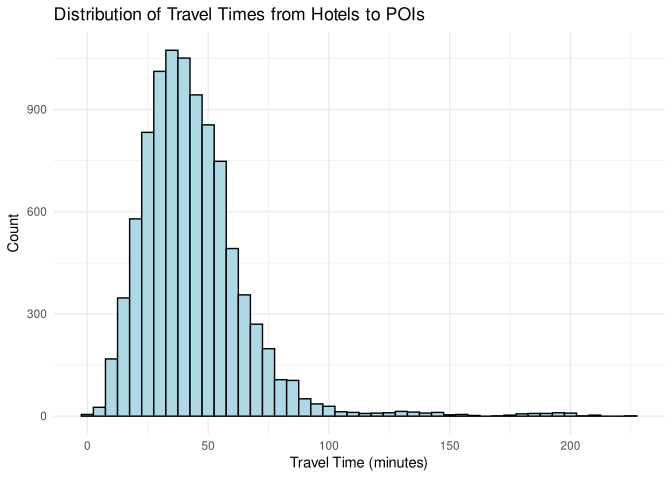
8 Merge Travel Times with Hotel Clusters
travel_times <- read.csv("data/berlin_hotel_poi_travel_times.csv")

hotels_h3_joined <- hotels_h3 |>
  left_join(
    travel_times,
    by = "origin"
  )

hotels_h3_joined |> saveRDS("data/berlin_hotels_with_travel_times.rds")
9 Scenarios
The three scenarios model different traveller preference profiles: a weighted random sample across all POI classes, museums and theatres only, and attractions and nightclubs only. Hotel rankings change substantially between scenarios. A hotel in Prenzlauer Berg performs well for nightlife (transit spread across the city) but mediocrely for museums (which cluster in Mitte, favouring more central locations). Charlottenburg shows the opposite pattern.
hotels_h3_joined <- readRDS("data/berlin_hotels_with_travel_times.rds")

# Scenario 1: Weighted random sample of 7 POIs across all classes
set.seed(123)
preferred_pois <- berlin_pois |>
  sample_n(7, weight = user_ratings_total) |> select(dest)
The visualisation uses inverse distance weighting (IDW) interpolation over hex centroids to produce a continuous travel time surface, then draws isolines at 5-minute intervals. IDW assumes that accessibility at any unsampled point is a weighted average of the sampled hex centroids around it, with weight falling off as a power of distance. It doesn’t extrapolate well beyond the data boundary, which is why the interpolated surface is clipped to the convex hull of the hotel cluster before plotting — no phantom isolines in unpopulated areas.
A note on the grid resolution: dx = 0.005 (approximately 500m at Berlin’s latitude) is a deliberate tradeoff — finer grids improve isoline detail but increase IDW computation time roughly quadratically. At dx = 0.001 the contours are noticeably smoother; at dx = 0.005 they run in acceptable time for an exploratory analysis.
The IDW grid is created in EPSG:4326 (degrees), then transformed to EPSG:3857 (metres) to align with the OSM base tile from annotation_map_tile.
The red circles at 1 km, 3 km, and 5 km from the geographic centre make the core argument visual: some of the best-performing locations in Scenario 3 sit well outside the 5 km ring.
library(ggplot2)
library(sf)
library(ggspatial)
library(gstat)
library(stars)
library(metR)
library(dplyr)

plot_sample_map <- function(sampled_pois) {
  # 1. Data Preparation
  hotels_h3_sample <- hotels_h3_joined |>
    inner_join(sampled_pois, by = c("destination" = "dest")) |>
    group_by(h3_index, hotel_count, geometry) |>
    summarise(avg_travel_time = mean(time), .groups = "drop") |>
    filter(avg_travel_time < quantile(avg_travel_time, 0.9)) |>
    st_as_sf()

  poi_data <- berlin_pois |>
    inner_join(sampled_pois, by = "dest") |>
    st_as_sf()

  # 2. Interpolation for Isolines
  hotel_hull <- st_convex_hull(st_union(hotels_h3_sample))
  grid <- hotels_h3_sample |>
    st_bbox() |>
    st_as_stars(dx = 0.005, dy = 0.005) |>
    st_set_crs(4326)

  idw_df <- idw((avg_travel_time / 60) ~ 1, hotels_h3_sample, grid) |>
    st_as_sf(as_points = TRUE) |>
    st_filter(hotel_hull) |>
    st_transform(3857)

  idw_df$x <- st_coordinates(idw_df)[, 1]
  idw_df$y <- st_coordinates(idw_df)[, 2]
  idw_df <- as.data.frame(idw_df)

  # 3. Reference Geometry (1/3/5 km circles from geographic centre)
  berlin_center <- st_sfc(st_point(c(13.4050, 52.5200)), crs = 4326)
  circle_1km <- berlin_center |>
    st_transform(3035) |>
    st_buffer(1000) |>
    st_transform(3857)
  circle_3km <- berlin_center |>
    st_transform(3035) |>
    st_buffer(3000) |>
    st_transform(3857)
  circle_5km <- berlin_center |>
    st_transform(3035) |>
    st_buffer(5000) |>
    st_transform(3857)

  # 4. Plotting
  ggplot() +
    annotation_map_tile(type = "osm", zoom = 12, alpha = 0.7) +
    geom_sf(
      data = st_transform(hotels_h3_sample, 3857),
      aes(fill = avg_travel_time / 60),
      color = "#333333", linewidth = 0.1, alpha = 0.5
    ) +
    geom_contour(
      data = idw_df, aes(x = x, y = y, z = var1.pred),
      breaks = seq(0, 200, by = 5), color = "black", linewidth = 0.4
    ) +
    geom_text_contour(
      data = idw_df, aes(x = x, y = y, z = var1.pred),
      breaks = seq(0, 200, by = 5), stroke = 0.15, size = 2.5
    ) +
    geom_sf(
      data = st_transform(poi_data, 3857),
      aes(shape = fclass, color = fclass), size = 3
    ) +
    geom_sf(data = circle_1km, fill = NA, color = "red", linewidth = 0.5) +
    geom_sf(data = circle_3km, fill = NA, color = "red", linewidth = 0.5) +
    geom_sf(data = circle_5km, fill = NA, color = "red", linewidth = 0.5) +
    scale_fill_gradientn(
      colors = c("green", "yellow", "red"),
      name = "Time (min)"
    ) +
    scale_shape_manual(values = c(
      "attraction" = 17, "museum" = 15, "theatre" = 18,
      "nightclub" = 19, "ruins" = 8
    ), name = "POI Type") +
    scale_color_manual(values = c(
      "attraction" = "#E41A1C", "museum" = "#377EB8",
      "theatre" = "#4DAF4A", "nightclub" = "#984EA3", "ruins" = "#FF7F00"
    ), name = "POI Type") +
    guides(
      fill = guide_colorbar(order = 1),
      shape = guide_legend(order = 2),
      color = guide_legend(order = 2)
    ) +
    coord_sf(crs = 3857) +
    theme_minimal() +
    theme(
      axis.text = element_blank(),
      axis.title = element_blank()
    ) +
    labs(
      title = "Berlin Accessibility & Cultural POIs",
      subtitle = "Shaded hexagons with 5-minute travel time contours"
    )
}

plot_sample_map(preferred_pois)
[inverse distance weighted interpolation]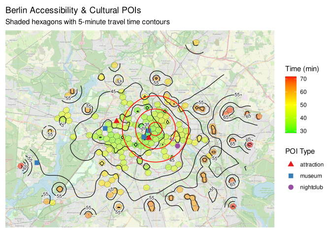
# Scenario 2: Focus on museums and theaters
preferred_pois <- berlin_pois |>
  filter(fclass %in% c("museum", "theatre")) |>
  sample_n(7, weight = user_ratings_total) |> select(dest)

plot_sample_map(preferred_pois)
[inverse distance weighted interpolation]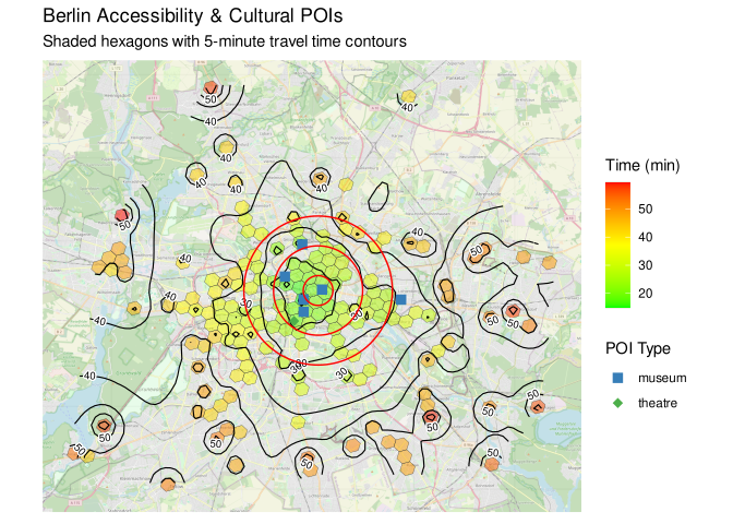
# Scenario 3: Focus on nightclubs and attractions
preferred_pois <- berlin_pois |>
  filter(fclass %in% c("attraction", "nightclub")) |>
  sample_n(7, weight = user_ratings_total) |> select(dest)

plot_sample_map(preferred_pois)
[inverse distance weighted interpolation]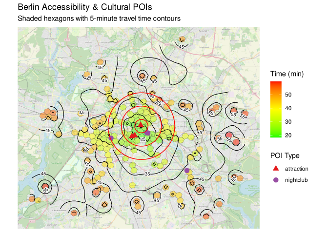
10 What’s Next
The proof of concept demonstrates the method. A production version would need:
Dynamic POI selection — let the user specify their points of interest rather than selecting from a fixed list of 50.
Departure time sensitivity — transit times in Berlin vary significantly between peak and off-peak hours; a morning departure to a museum is a different routing problem than a late-night return from a club.
Kano validation — conduct a research to validate the perceived value, see Kano Method for Prioritization of Features.
The full code is in the GitHub repository. The processed travel time data is included for reproducibility without re-running the API calls.
11 See Also
Here are some of my other posts related to R, geospatial analysis, and data visualization:


No matching items